Categorical Variables
Goal Make quantitative statements about qualitative information.
- e.g., race, gender, being employed, living in Oregon, etc.
Approach. Construct binary variables.
- a.k.a. dummy variables or indicator variables.
- Value equals 1 if observation is in the category or 0 if otherwise.
Regression implications.
Change the interpretation of the intercept.
Change the interpretations of the slope parameters.
Continuous Variables
Consider the relationship
\[
\text{Pay}_i = \beta_0 + \beta_1 \text{School}_i + u_i
\]
where
- \(\text{Pay}_i\) is a continuous variable measuring an individual’s pay
- \(\text{School}_i\) is a continuous variable that measures years of education
Interpretation
- \(\beta_0\): \(y\)-intercept, i.e., \(\text{Pay}\) when \(\text{School} = 0\)
- \(\beta_1\): expected increase in \(\text{Pay}\) for a one-unit increase in \(\text{School}\)
Consider the relationship
\[
\text{Pay}_i = \beta_0 + \beta_1 \text{School}_i + u_i
\]
Derive the slope’s interpretation.
\(\mathop{\mathbb{E}}\left[ \text{Pay} | \text{School} = \ell + 1 \right] - \mathop{\mathbb{E}}\left[ \text{Pay} | \text{School} = \ell \right]\)
\(\quad = \mathop{\mathbb{E}}\left[ \beta_0 + \beta_1 (\ell + 1) + u \right] - \mathop{\mathbb{E}}\left[ \beta_0 + \beta_1 \ell + u \right]\)
\(\quad = \left[ \beta_0 + \beta_1 (\ell + 1) \right] - \left[ \beta_0 + \beta_1 \ell \right]\)
\(\quad = \beta_0 - \beta_0 + \beta_1 \ell - \beta_1 \ell + \beta_1\) \(\: = \beta_1\).
Expected increase in pay for an additional year of schooling
Continuous Variables
Consider the relationship
\[
\text{Pay}_i = \beta_0 + \beta_1 \text{School}_i + u_i
\]
Alternative derivation:
Differentiate the model with respect to schooling:
\[
\dfrac{\partial \text{Pay}}{\partial \text{School}} = \beta_1
\]
Expected increase in pay for an additional year of schooling
If we have multiple explanatory variables, e.g.,
\[
\text{Pay}_i = \beta_0 + \beta_1 \text{School}_i + \beta_2 \text{Ability}_i + u_i
\]
then the interpretation changes slightly.
\(\mathop{\mathbb{E}}\left[ \text{Pay} | \text{School} = \ell + 1 \land \text{Ability} = \alpha \right] - \mathop{\mathbb{E}}\left[ \text{Pay} | \text{School} = \ell \land \text{Ability} = \alpha \right]\)
\(\quad = \mathop{\mathbb{E}}\left[ \beta_0 + \beta_1 (\ell + 1) + \beta_2 \alpha + u \right] - \mathop{\mathbb{E}}\left[ \beta_0 + \beta_1 \ell + \beta_2 \alpha + u \right]\)
\(\quad = \left[ \beta_0 + \beta_1 (\ell + 1) + \beta_2 \alpha \right] - \left[ \beta_0 + \beta_1 \ell + \beta_2 \alpha \right]\)
\(\quad = \beta_0 - \beta_0 + \beta_1 \ell - \beta_1 \ell + \beta_1 + \beta_2 \alpha - \beta_2 \alpha\) \(\: = \beta_1\)
The slope gives the expected increase in pay for an additional year of schooling, holding ability constant.
Continuous Variables
If we have multiple explanatory variables, e.g.,
\[
\text{Pay}_i = \beta_0 + \beta_1 \text{School}_i + \beta_2 \text{Ability}_i + u_i
\]
then the interpretation changes slightly.
Alternative derivation
Differentiate the model with respect to schooling:
\[
\dfrac{\partial\text{Pay}}{\partial\text{School}} = \beta_1
\]
The slope gives the expected increase in pay for an additional year of schooling, holding ability constant.
Categorical Variables
Consider the relationship
\[
\text{Pay}_i = \beta_0 + \beta_1 \text{Female}_i + u_i
\]
where \(\text{Pay}_i\) is a continuous variable measuring an individual’s pay and \(\text{Female}_i\) is a binary variable equal to \(1\) when \(i\) is female.
Interpretation of \(\beta_0\)
\(\beta_0\) is the expected \(\text{Pay}\) for males (i.e., when \(\text{Female} = 0\)):
\[
\mathop{\mathbb{E}}\left[ \text{Pay} | \text{Male} \right] = \mathop{\mathbb{E}}\left[ \beta_0 + \beta_1\times 0 + u_i \right] = \mathop{\mathbb{E}}\left[ \beta_0 + 0 + u_i \right] = \beta_0
\]
Categorical Variables
Consider the relationship
\[
\text{Pay}_i = \beta_0 + \beta_1 \text{Female}_i + u_i
\]
where \(\text{Pay}_i\) is a continuous variable measuring an individual’s pay and \(\text{Female}_i\) is a binary variable equal to \(1\) when \(i\) is female.
Interpretation of \(\beta_1\)
\(\beta_1\) is the expected difference in \(\text{Pay}\) between females and males:
\(\mathop{\mathbb{E}}\left[ \text{Pay} | \text{Female} \right] - \mathop{\mathbb{E}}\left[ \text{Pay} | \text{Male} \right]\)
\(\quad = \mathop{\mathbb{E}}\left[ \beta_0 + \beta_1\times 1 + u_i \right] - \mathop{\mathbb{E}}\left[ \beta_0 + \beta_1\times 0 + u_i \right]\)
\(\quad = \mathop{\mathbb{E}}\left[ \beta_0 + \beta_1 + u_i \right] - \mathop{\mathbb{E}}\left[ \beta_0 + 0 + u_i \right]\)
\(\quad = \beta_0 + \beta_1 - \beta_0\) \(\quad = \beta_1\)
Categorical Variables
Consider the relationship
\[
\text{Pay}_i = \beta_0 + \beta_1 \text{Female}_i + u_i
\]
where \(\text{Pay}_i\) is a continuous variable measuring an individual’s pay and \(\text{Female}_i\) is a binary variable equal to \(1\) when \(i\) is female.
Interpretation
\(\beta_0 + \beta_1\): is the expected \(\text{Pay}\) for females:
\(\mathop{\mathbb{E}}\left[ \text{Pay} | \text{Female} \right]\)
\(\quad = \mathop{\mathbb{E}}\left[ \beta_0 + \beta_1\times 1 + u_i \right]\)
\(\quad = \mathop{\mathbb{E}}\left[ \beta_0 + \beta_1 + u_i \right]\)
\(\quad = \beta_0 + \beta_1\)
Categorical Variables
Consider the relationship
\[
\text{Pay}_i = \beta_0 + \beta_1 \text{Female}_i + u_i
\]
Interpretation
- \(\beta_0\): expected \(\text{Pay}\) for males (i.e., when \(\text{Female} = 0\))
- \(\beta_1\): expected difference in \(\text{Pay}\) between females and males
- \(\beta_0 + \beta_1\): expected \(\text{Pay}\) for females
- Males are the reference group
Categorical Variables
Consider the relationship
\[
\text{Pay}_i = \beta_0 + \beta_1 \text{Female}_i + u_i
\]
Note. If there are no other variables to condition on, then \(\hat{\beta}_1\) equals the difference in group means, e.g., \(\bar{X}_\text{Female} - \bar{X}_\text{Male}\).
Note2. The holding all other variables constant interpretation also applies for categorical variables in multiple regression settings.
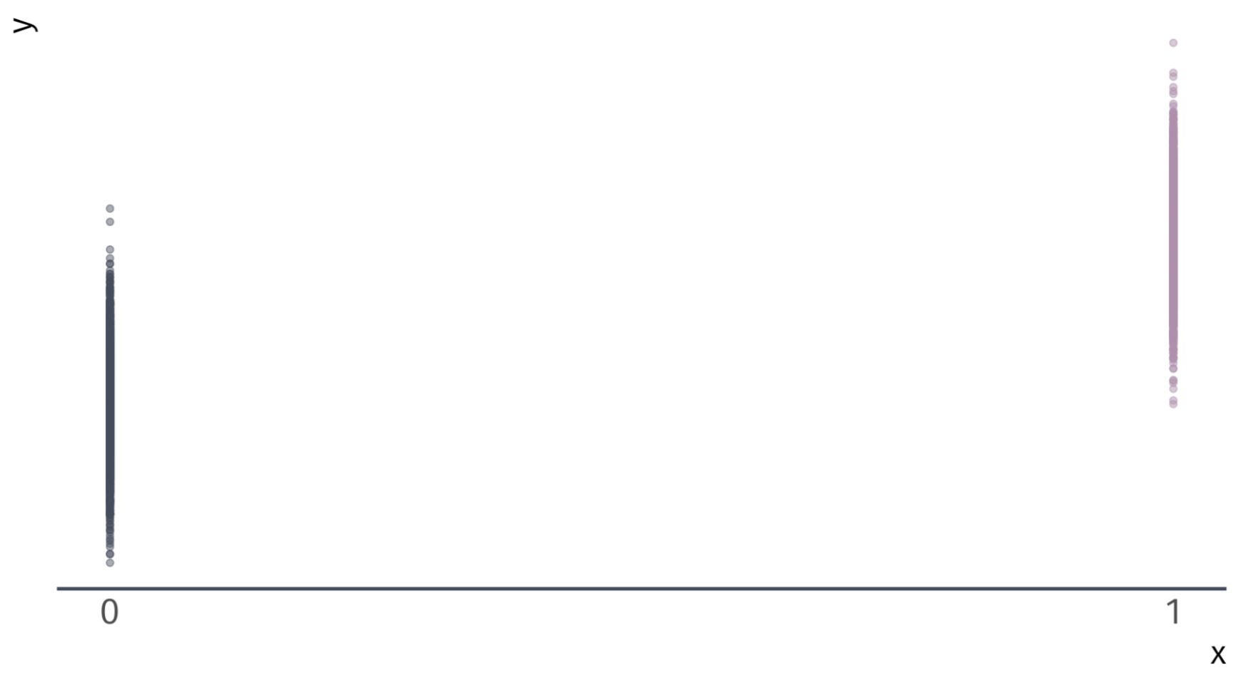
Categorical Variables
\(Y_i = \beta_0 + \beta_1 X_i + u_i\) for binary variable \(X_i = \{\color{#434C5E}{0}, \, {\color{#B48EAD}{1}}\}\)
![]()
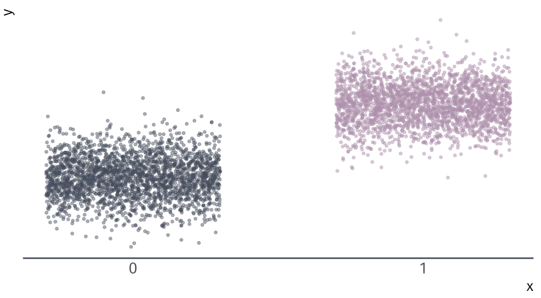
Categorical Variables
\(Y_i = \beta_0 + \beta_1 X_i + u_i\) for binary variable \(X_i = \{\color{#434C5E}{0}, \, {\color{#B48EAD}{1}}\}\)
![]()
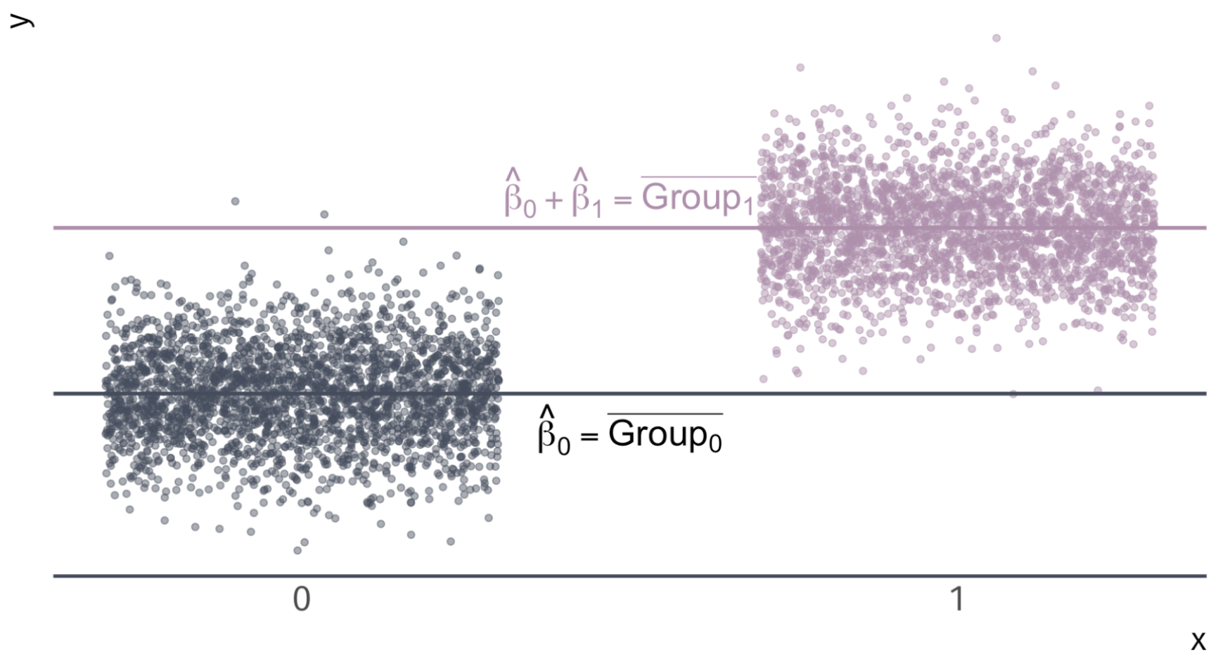
Categorical Variables
\(Y_i = \beta_0 + \beta_1 X_i + u_i\) for binary variable \(X_i = \{\color{#434C5E}{0}, \, {\color{#B48EAD}{1}}\}\)
![]()
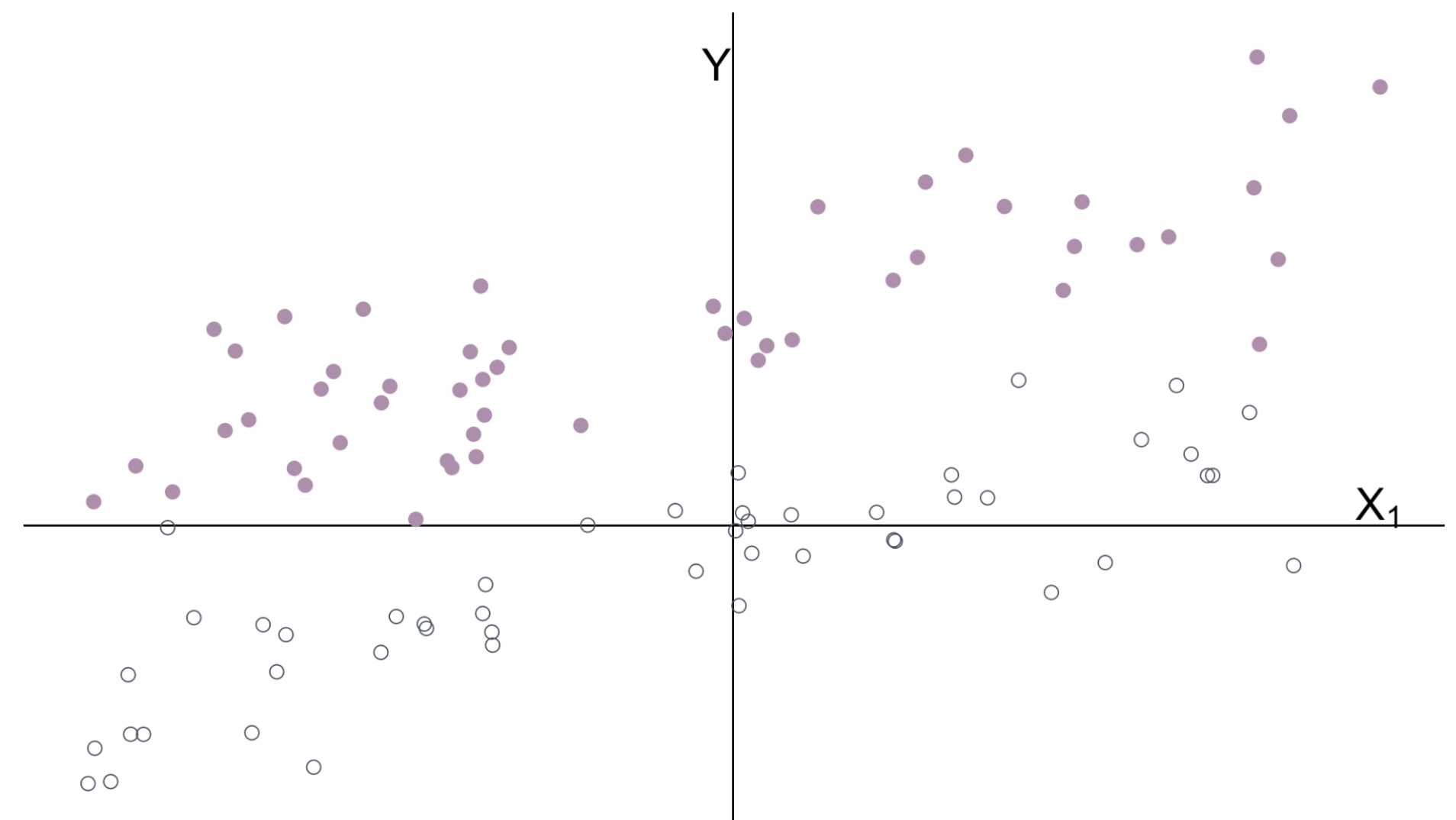
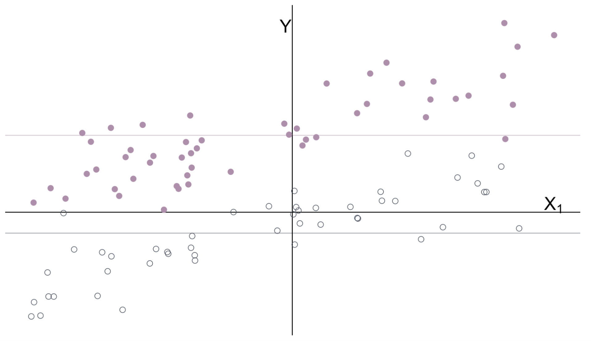
Multiple Regression
\(Y_i = \beta_0 + \beta_1 X_{1i} + \beta_2 X_{2i} + u_i \quad\) \(X_1\) is continuous \(\quad X_2\) is categorical
![]()
Multiple Regression
The intercept and categorical variable \(X_2\) control for the groups’ means.
![]()
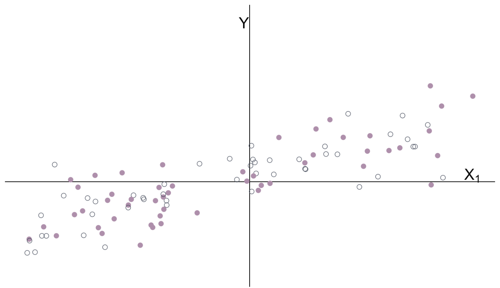
Multiple Regression
With groups’ means removed
![]()
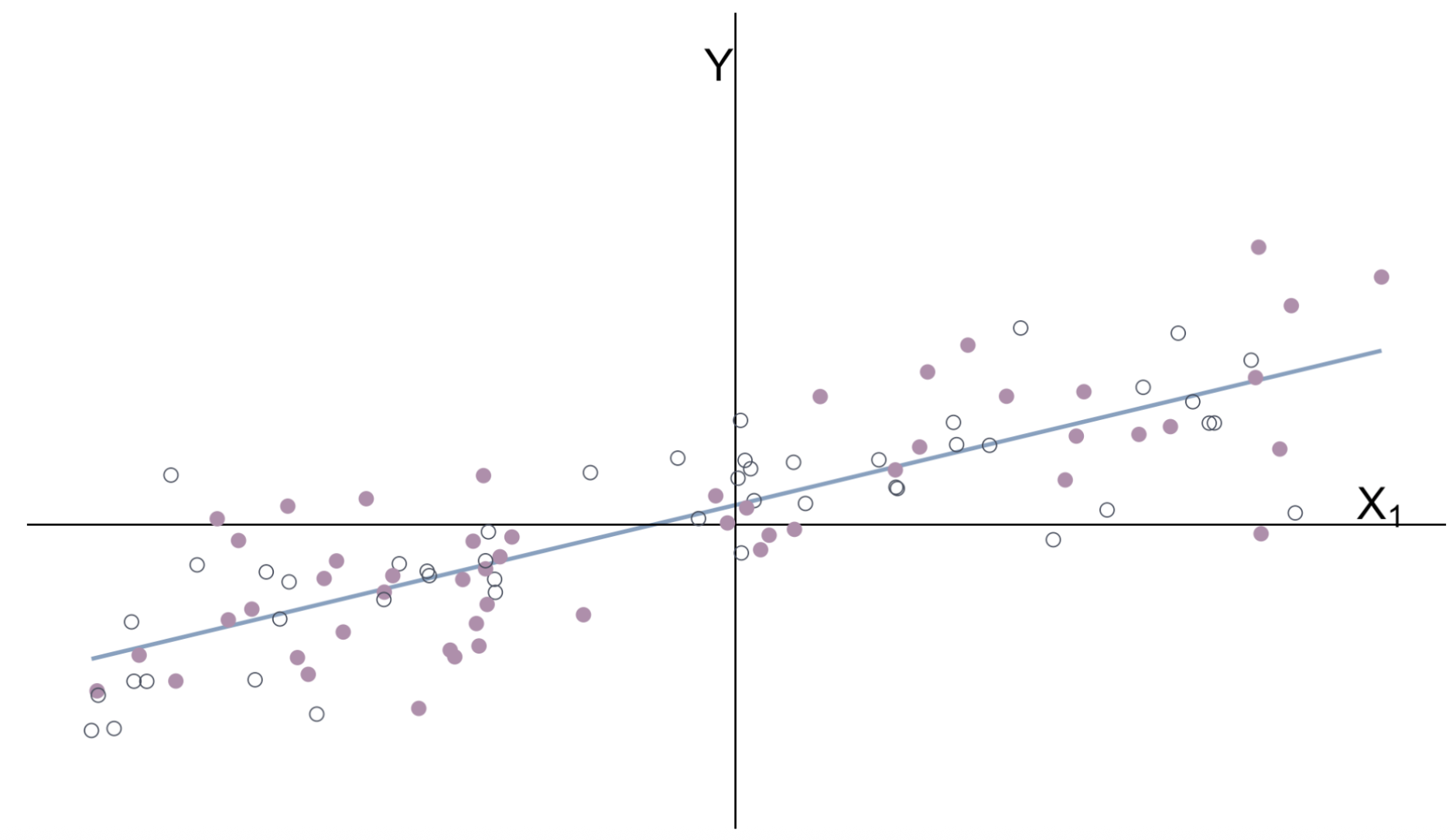
Multiple Regression
\(\hat{\beta}_1\) estimates the relationship between \(Y\) and \(X_1\) after controlling for \(X_2\).
![]()
Multiple Regression
Another way to think about it: Regression by group
![]()
Omitted Variable Bias Example
Omitted variable bias
Ex. Imagine a population model for the amount individual \(i\) gets paid
\[
\text{Pay}_i = \beta_0 + \beta_1 \text{School}_i + \beta_2 \text{Male}_i + u_i
\]
where \(\text{School}_i\) gives \(i\)’s years of schooling and \(\text{Male}_i\) denotes an indicator variable for whether individual \(i\) is male.
Interpretation
- \(\beta_1\): returns to an additional year of schooling (ceteris paribus)
- \(\beta_2\): premium for being male (ceteris paribus)
If \(\beta_2 > 0\), then there is discrimination against women.
Omitted variable bias
Ex. From the population model
\[
\text{Pay}_i = \beta_0 + \beta_1 \text{School}_i + \beta_2 \text{Male}_i + u_i
\]
An analyst focuses on the relationship between pay and schooling, i.e.,
\[
\text{Pay}_i = \beta_0 + \beta_1 \text{School}_i + \left(\beta_2 \text{Male}_i + u_i\right)
\] \[
\text{Pay}_i = \beta_0 + \beta_1 \text{School}_i + \varepsilon_i
\]
where \(\varepsilon_i = \beta_2 \text{Male}_i + u_i\).
Omitted variable bias
We assumed exogeniety to show that OLS is unbiased.
Even if \(\mathop{\mathbb{E}}\left[ u | X \right] = 0\), it is not necessarily true that \(\mathop{\mathbb{E}}\left[ \varepsilon | X \right] = 0\)
- If \(\beta_2 \neq 0\), then it is false
Specifically, if
\[
\mathop{\mathbb{E}}\left[ \varepsilon | \text{Male} = 1 \right] = \beta_2 + \mathop{\mathbb{E}}\left[ u | \text{Male} = 1 \right] \neq 0
\]
Omitted Variable Bias
Let’s try to see this result graphically.
The true population model:
\[
\text{Pay}_i = 20 + 0.5 \times \text{School}_i + 10 \times \text{Male}_i + u_i
\]
The regression model that suffers from omitted-variable bias:
\[
\text{Pay}_i = \hat{\beta}_0 + \hat{\beta}_1 \times \text{School}_i + e_i
\]
Suppose that women, on average, receive more schooling than men.
Omitted Variable Bias
True model: \(\text{Pay}_i = 20 + 0.5 \times \text{School}_i + 10 \times \text{Male}_i + u_i\)
![]()
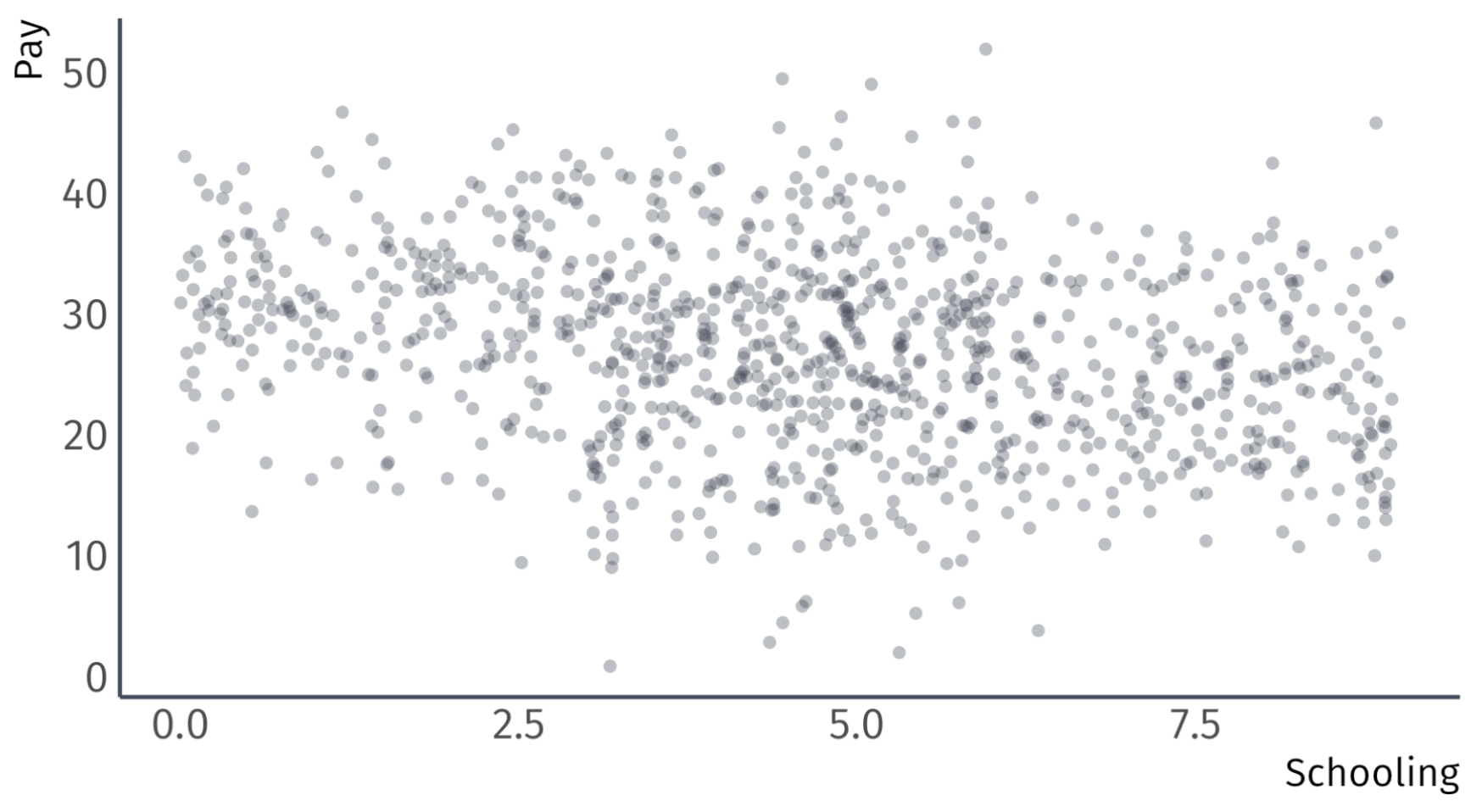
Omitted Variable Bias
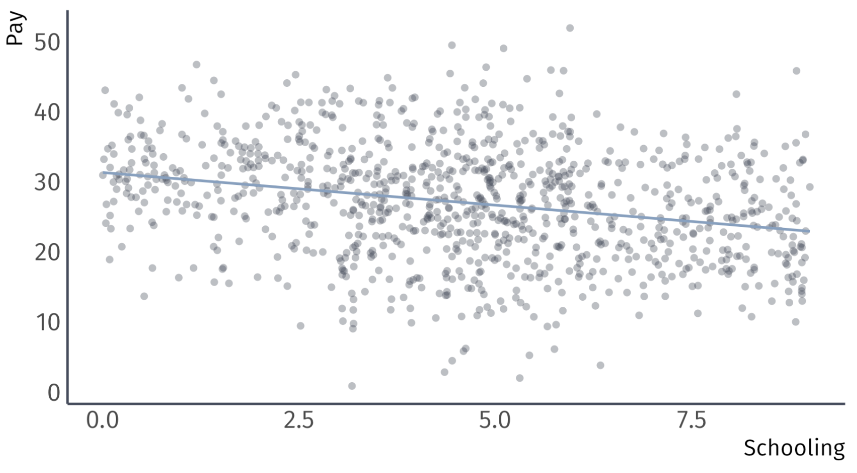
Biased regression: \(\widehat{\text{Pay}}_{i} = 31.3 - 0.9 \times \text{School}_{i}\)
![]()
Omitted Variable Bias
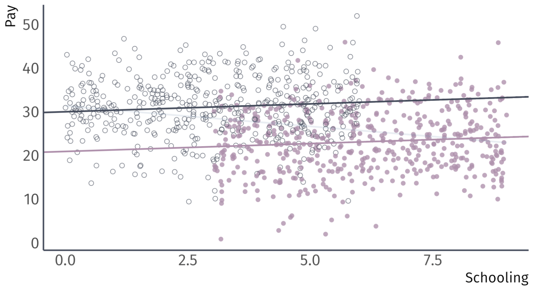
Recalling the omitted variable: Sex (female vs male)
![]()
Omitted Variable Bias
Recalling the omitted variable: Sex (female vs male)
![]()
Omitted Variable Bias
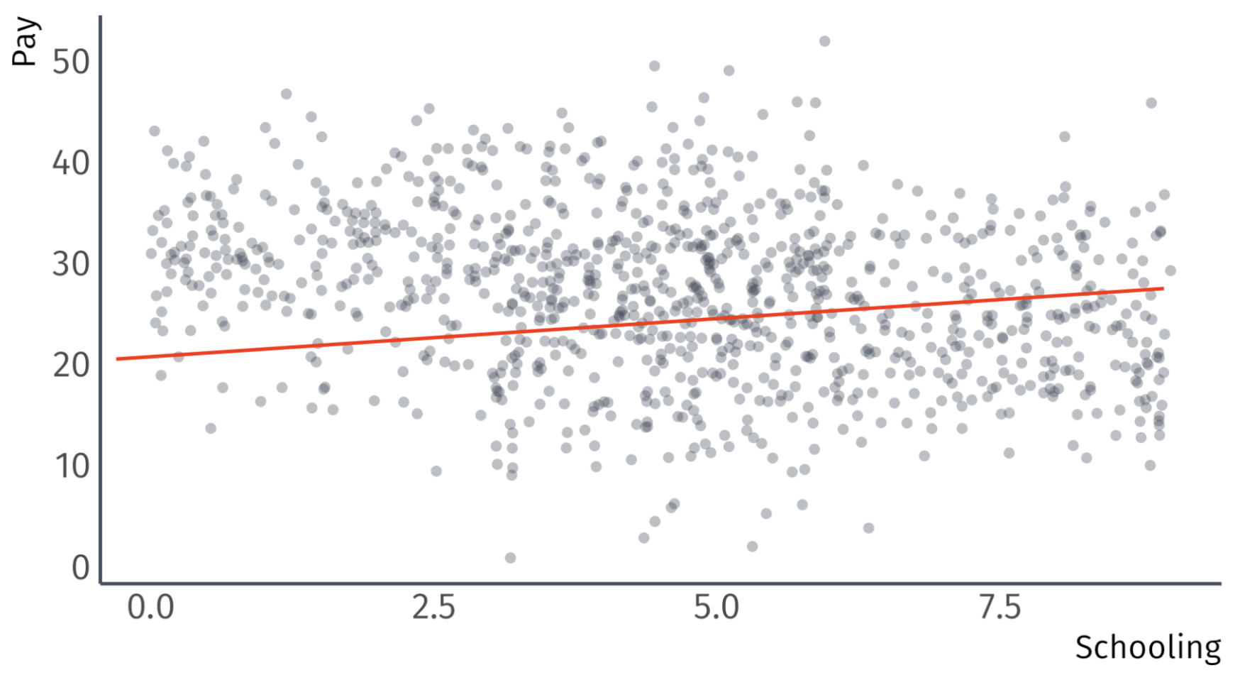
Unbiased Regression:
\[
\widehat{\text{Pay}}_{i} = 20.9 + 0.4 \times \text{School}_{i} + 9.1 \times \text{Male}_{i}
\]
![]()