Data manipulation and querying is a very useful skill.
An equally important one is being able to visualize the data.
In this lecture, you will learn a handful of recipes to draw plots using ggplot
In particular, you will learn about:
Bar plots
Histograms
Box plots (“Box-and-Whisker” plots)
Scatterplots (and how to add a best fit line)
Recipes for Success
But First…
We need some data.
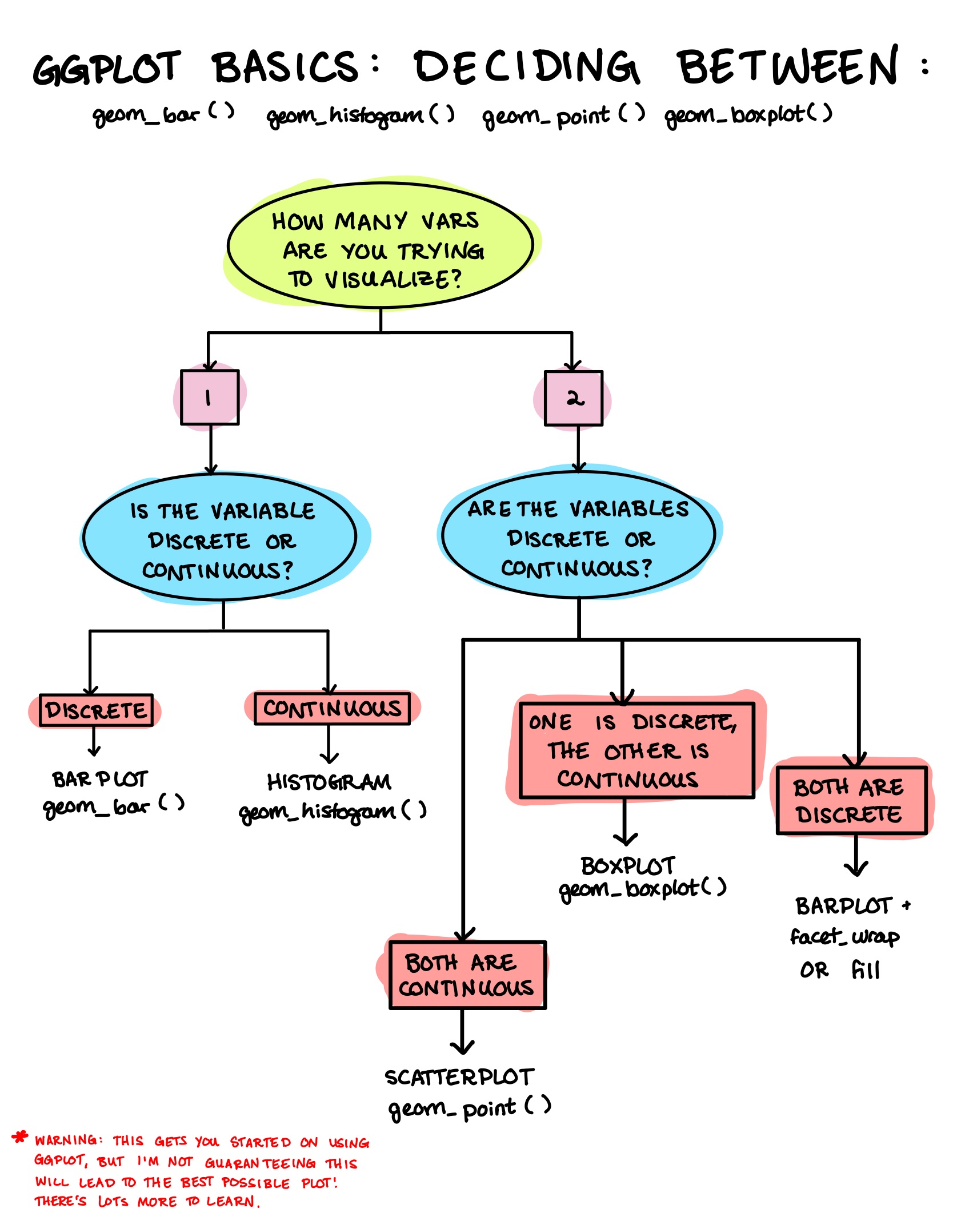
As you’ll see, the type of plot you will want to draw depends crucially on the type of data that you have.
Suppose we have a tibble called students that looks like this:
sex
study_time
grade1
final_grade
female
5-10 hrs
94.9
95.4
male
2-5 hrs
79.6
73.7
female
5-10 hrs
64.2
49.1
. . .
. . .
. . .
. . .
Where study_time is hours per week studying math, grade1 is their first-semester math grade, and final_grade is their final grade in the math course
But First…
sex
study_time
grade1
final_grade
female
5-10 hrs
94.9
95.4
male
2-5 hrs
79.6
73.7
female
5-10 hrs
64.2
49.1
. . .
. . .
. . .
. . .
We have some variables which are categorical (sex takes either “male” or “female” and study_time takes on 0-2 hrs, 2-5 hrs, etc.).
We have other variables which are numeric, and in particular, continuous (grade1 and final_grade can take any value between 0 and 100)
These being different “type” of variables means we use different “recipes” to visualize them
Data and quick ggplot() syntax
I will be using the dataset you can find below the lecture, named students
Download it, open RStudio and in your terminal load it using:
load("./students-data.Rdata")
The exact path will change depending on where it is stored on your device. I recommend right-clicking on the file itself and copying the path shown in the properties.
Note: This is not necessary for you to do. It’s just if you want to follow along
Recipe 1: Bar Plots
geom_bar()
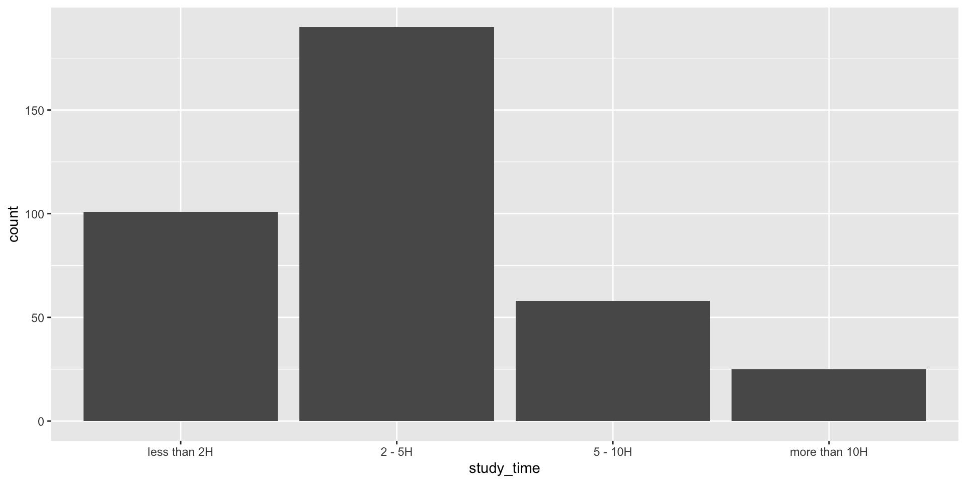
Q:How many hours do students spend studying?
Distrubtion of a single discrete variable \(\rightarrow\) Use a Bar Plot
students %>%ggplot(aes(x = study_time)) +geom_bar()
Here I pipe the tibble into the function ggplot()
ggplot() needs an aesthetic mapping. You need to tell it which variables in your dataset map to which visual aesthetic in the plot.
After the ggplot() call, add any extra layer with +
geom_bar() draws the bar plot using the previous instructions
students %>%ggplot(aes(x = study_time)) +geom_bar()
Which admittedly looks ugly but we can spice it up later
Recipe 2: Histograms
geom_histogram()
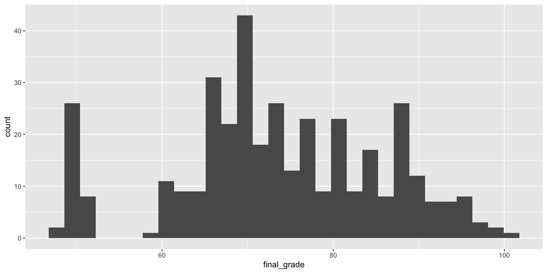
Q:What is the grade distribution?
Distribution of a single continuous variable \(\rightarrow\) use a histogram
The recipe remains largely the same: Pipe the data into ggplot(), then ggplot() needs an aesthetic mapping which is wrapped in aes().
Then use the specific geom_histogram() to draw the histogram.
students %>%ggplot(aes(x = final_grade)) +geom_histogram()
students %>%ggplot(aes(x = final_grade)) +geom_histogram()
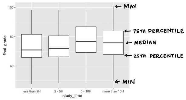
Recipe 3: Box Plots
geom_boxplot()
Q.Do students who study more (discrete) earn higher grades (continuous)?
Begin by piping the data into ggplot()
Provide ggplot() the aesthetic wrapped in aes()
This time we have 2 variables: one for each axis
students %>%ggplot(aes(x = study_time, y = final_grade)) +geom_boxplot()
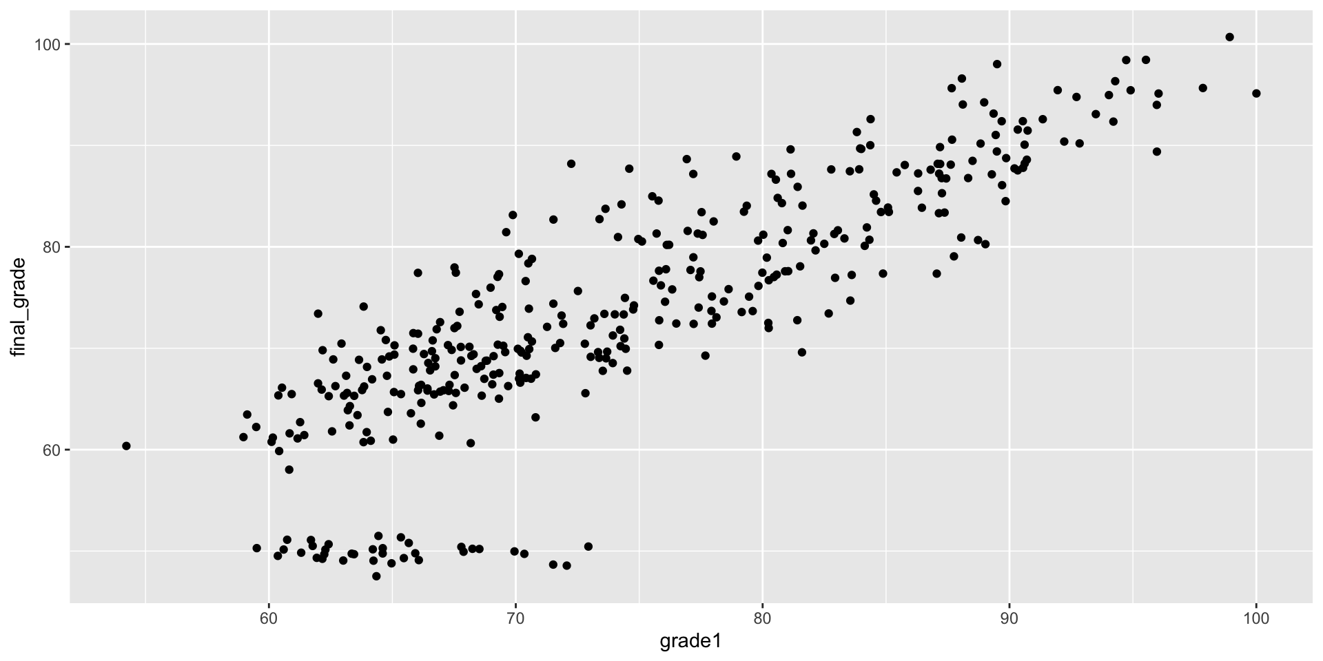
Recipe 4: Scatterplots
geom_point()
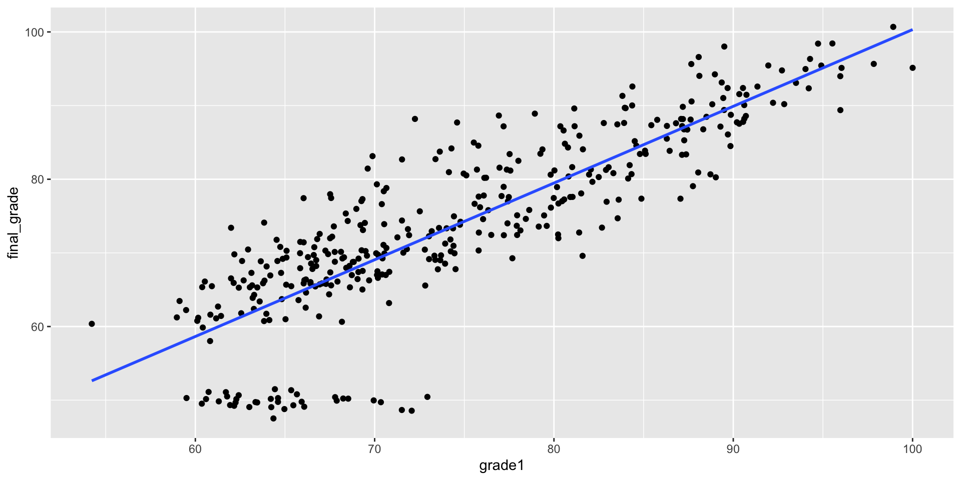
Q.How well does a student’s first-semester grade predict their final grade in a (high school) class?
students %>%ggplot(aes(x = grade1, y = final_grade)) +geom_point()
students %>%ggplot(aes(x = grade1, y = final_grade)) +geom_point()
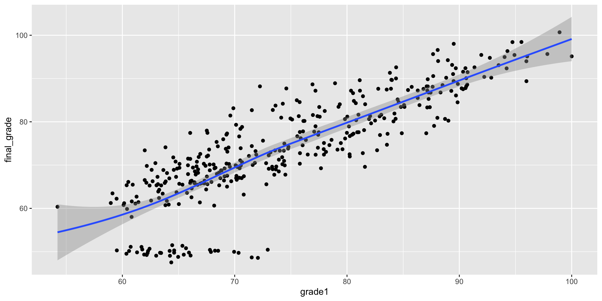
Which looks fine, but what about adding an additional layer: a best fit line
students %>%ggplot(aes(x = grade1, y = final_grade)) +geom_point() +geom_smooth()
We can further modify our geom_smooth line to make it a linear model using method = "lm" and also remove the predicted standard errors se=FALSE
students %>%ggplot(aes(x = grade1, y = final_grade)) +geom_point() +geom_smooth(method ="lm", se =FALSE)
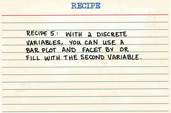
Recipe 5: Bar Plots
geom_bar()
Q.Do females report studying for longer than males?
Relationship between time studied and sex
We can do this in two different ways:
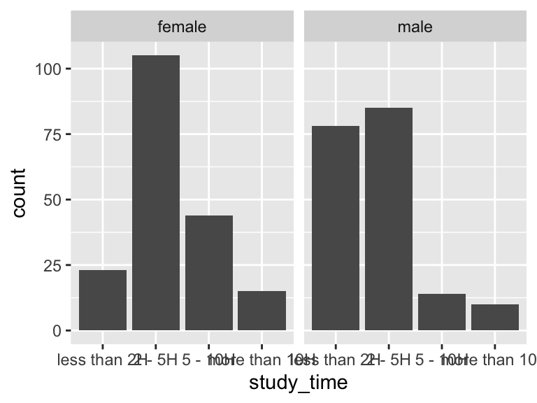
Make a bar plot for each category (sex) which creates separate plots
students %>%ggplot(aes(x = study_time)) +geom_bar() +facet_wrap(~ sex) # ~ indicates a formula is coming
Recipe 5: Bar Plots
geom_bar()
Q.Do females report studying for longer than males?
Relationship between time studied and sex
We can do this in two different ways:
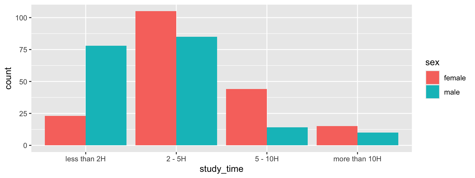
Try a fill aesthetic mapping to color in the bars using seperate colors for males and females
students %>%ggplot(aes(x = study_time, fill = sex)) +# Be sure to include the fill inside the aes()geom_bar(position ='dodge') # Use position = "dodge" to set bars next to each other. The default is to stack them on top of each other
A Few More Tools
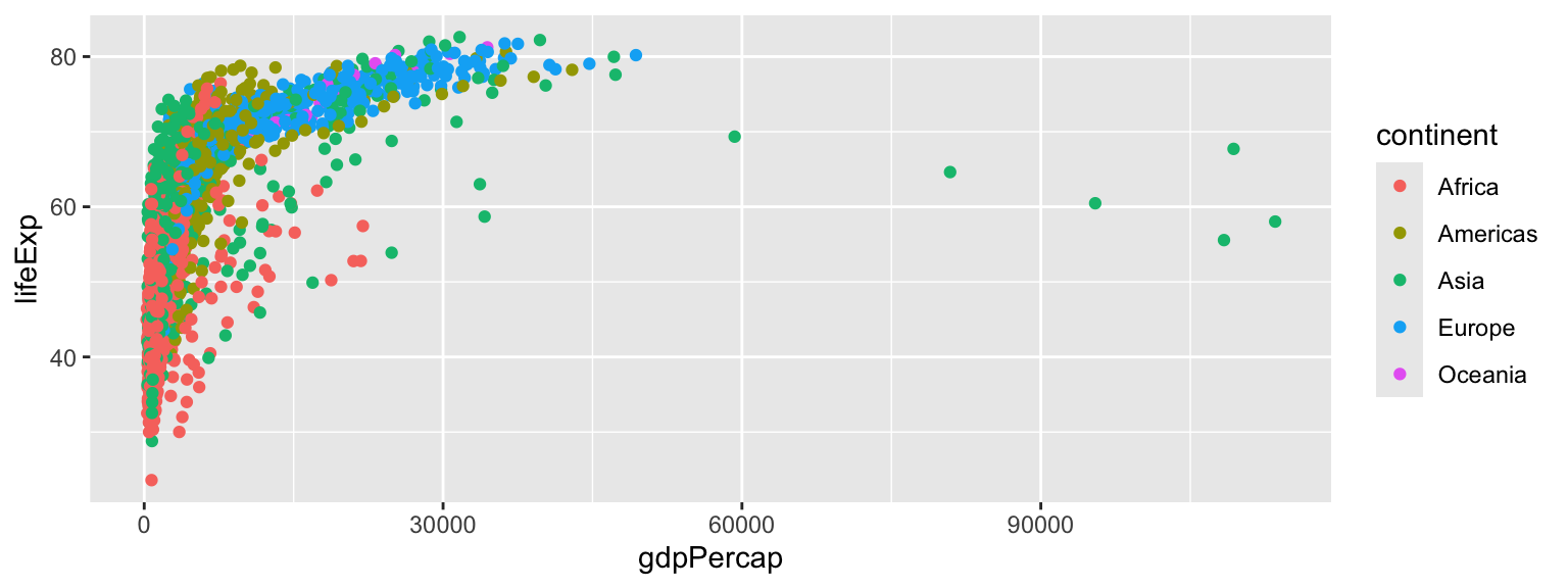
Say we want to show a scatterplot and have it differentiate amongst categories using different colors. It is very similar to fill =, but instead we use color =.
library(gapminder)gapminder %>%ggplot(aes(x = gdpPercap, y = lifeExp, color = continent)) +geom_point()
A Few More Tools
Summary
Aesthetic mappings get wrapped in aes() and map variables in your tibble to aesthetics in your plot like which variable gets drawn on the x-axis, which goes on the y-axis, and which variable is represented in color
Geoms are added to the plot using + as layers
Practice: Download “Worksheet 04” From the Site
This worksheet will help you learn coding by doing. You will:
Practice aesthetic mappings and all the recipes you’ve seen in this section