Factor Endowments | Heckscher-Ohlin Model

EC 380 - International Economic Issues

Jose Rojas-Fallas

2025

Heckscher-Ohlin Model

Introduction

The HO model starts by noting that countries are endowed with different levels of each input (factors)

Each output (goods) require a different technology and mixes of the various possibl inputs

Take for example coffee production. It requires:

• Coffee plants
• Workers to harvest

• Expensive and large ovens
• Engineers and “Q Graders”

The fact that some countries may inherently have higher availability of inputs creates productivity differences

HO Model - Key Terms

We define factors as inputs required in the production process

The fact that factors may be different introduces two relative measure definitions:

• Factor Abundance: If a particular factor \(X\) represents a large share of total factors, the country is \(X\)-factor abundant
• Factor Scarcity: If a country has less of a particular factor \(X\) relative to other factors, the country is \(X\)-factor scarce

In the HO model we will assume two factors of production:

Labor

Capital

HO Model - Key Terms

Since we have two factors, we can create a tool to compare them across countries:

The Capital-Labor Ratio allows us to assign countries into resource endowment groups

It is calculated as:

\[ \dfrac{\text{Capital}}{\text{Labor}} = \dfrac{K}{L} \]

The higher \(K/L\) is for a given country, relative to other countries, the more capital abundant it is

HO Model - Key Terms

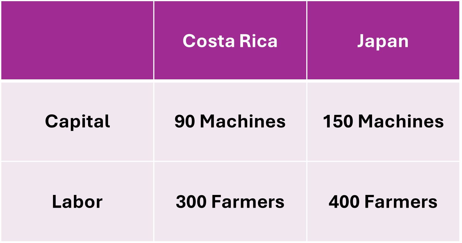
Which country is capital abundant?

Using the Capital-Labor Ratio we get

\[ \dfrac{K_{crc}}{L_{crc}} = 0.3 \;\;\;\; ; \;\;\;\; \dfrac{K_{jap}}{L_{jap}} = 0.375 \]

HO Model - Key Terms

The Capital-Labor Ratio implies factor abundancy

The country with the higher C-L ratio is relatively more abundant in capital

The country with the lower C-L ratio is relatively more abundant in labor

This also has implications for factor prices:

Countries where a given factor is relatively more abundant exhibit lower input prices per unit of the factor

A labor-abundant country finds labor to be relatively cheaper (per unit) than the capital-abundant country

It has a comparative advantage in labor-intensive production due to its edge in labor-costs

HO Model - Trade Theory

The Heckscher-Ohlin Model asserts that a country’s comparative advantage lies in the production on goods that intensively use relatively abundant factors

This may explain US trade patterns in which capital-intensive exports of jet engines and agricultural products dominate its goods outflows

• These goods are produced with a lot of physical capital and low amounts of high-skill labor (scientific, engineering, etc.)

Autarky & Trade

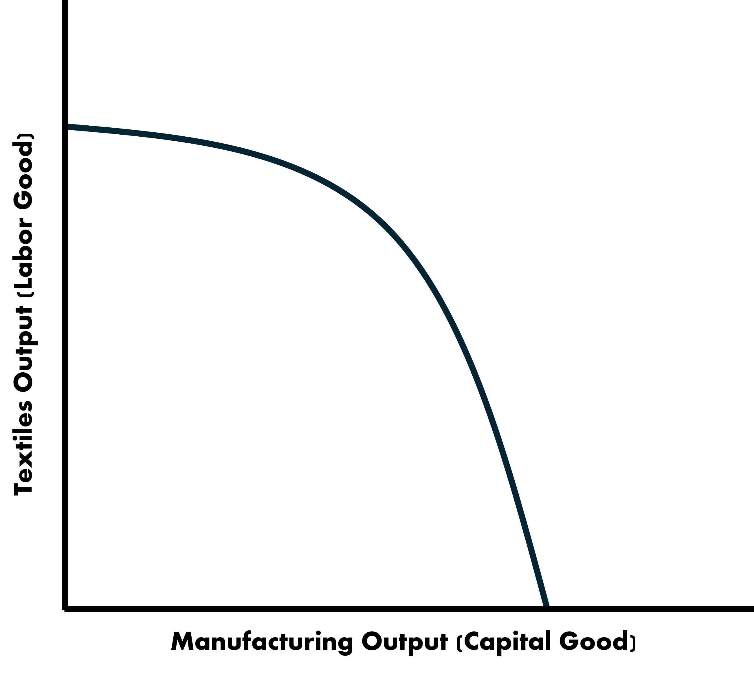
Production Possibilities Frontiers

The Ricardian Model assumed a single factor of production (labor) which was homogenous

• This implied that countries face the same trade-off between goods regardless of input levels

• The PPF was a straight line

The HO Model now considers combinations of factors where some specific mix of the two is most productive

• Because of this necessary mix of inputs, the PPF will be a curve

New PPF

PPF for Country A

New PPF - Increase in Labor Intensive Good

New PPF - Increase in Capital Intensive Good

New PPF

Adjustments at the extremes of the frontiers require a disproportionately large exchange in factors

• Each unit increase in one factor-good leads to an increasingly sizeable loss of the other factor-good
• Opportunity costs are rising for each type of production
• Why?

As you reallocate resources from a capital-intensive good to a labor-intensive, you need greater amounts of factors due to factor combinations being misaligned

• AKA It is not a linear trade-off

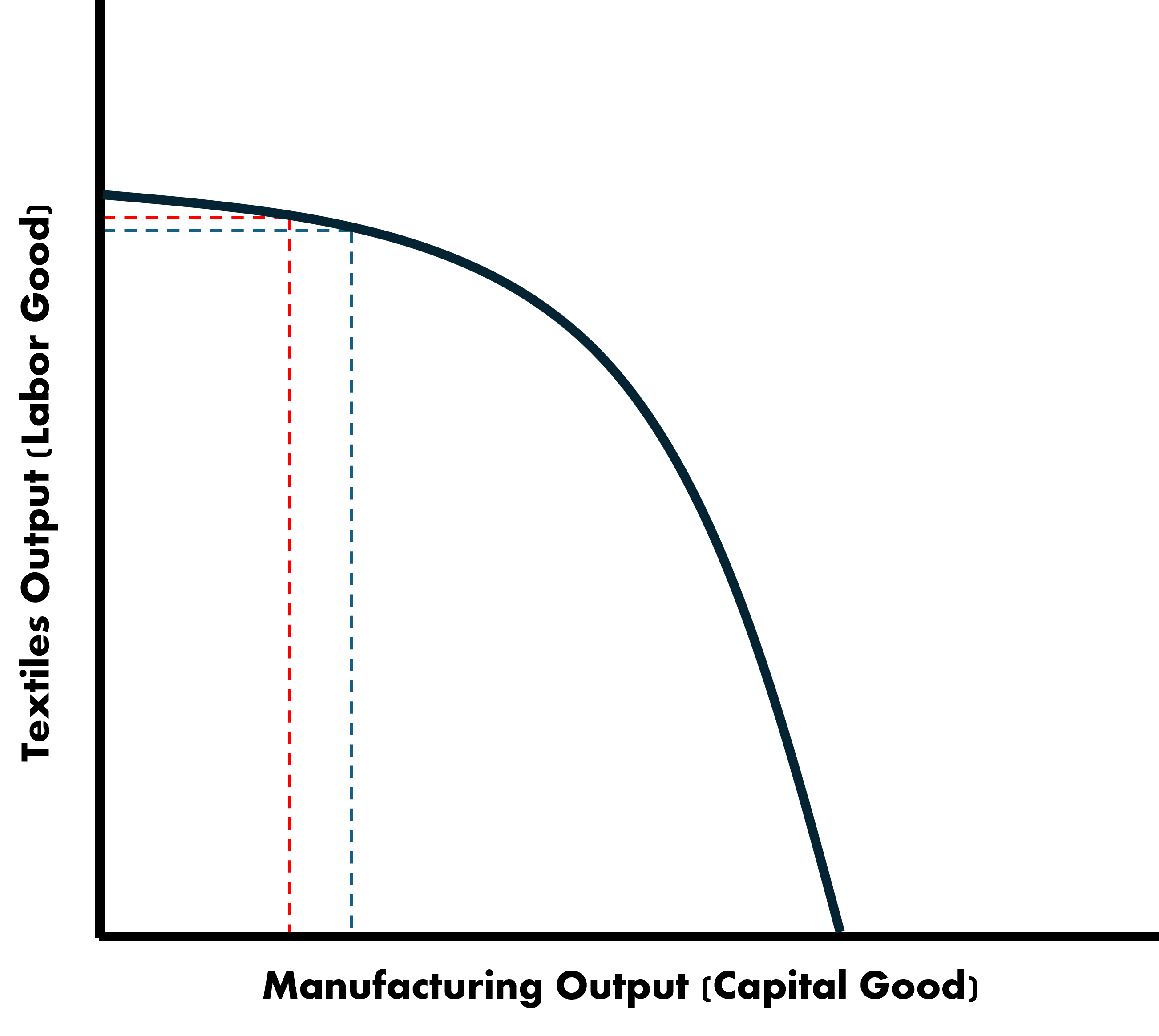
Autarky

country consumes exactly what it produces

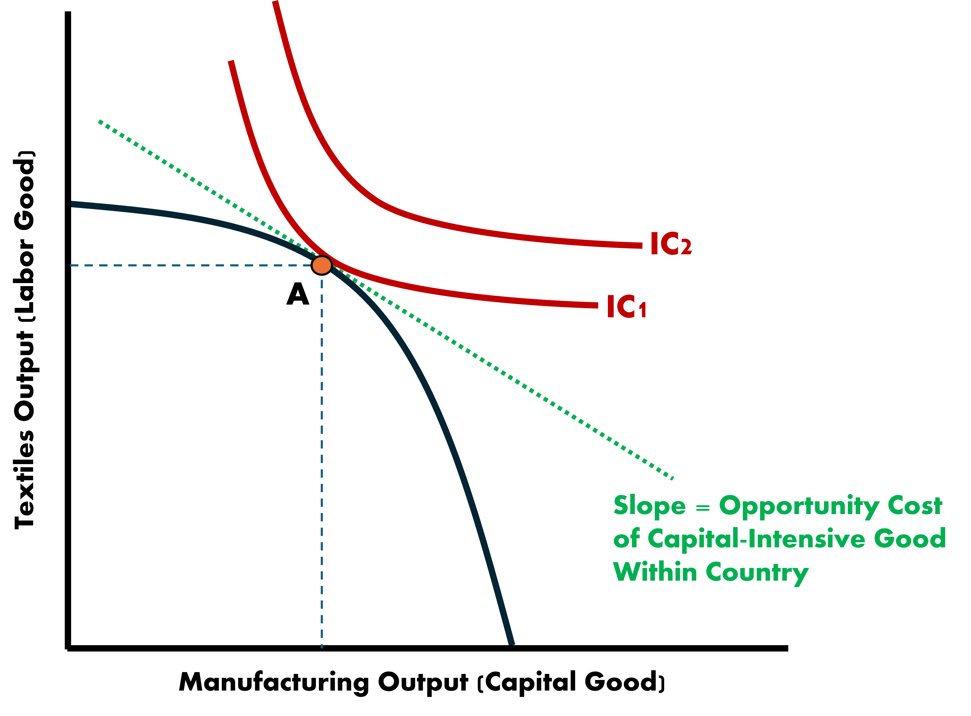
Free Trade - World Price

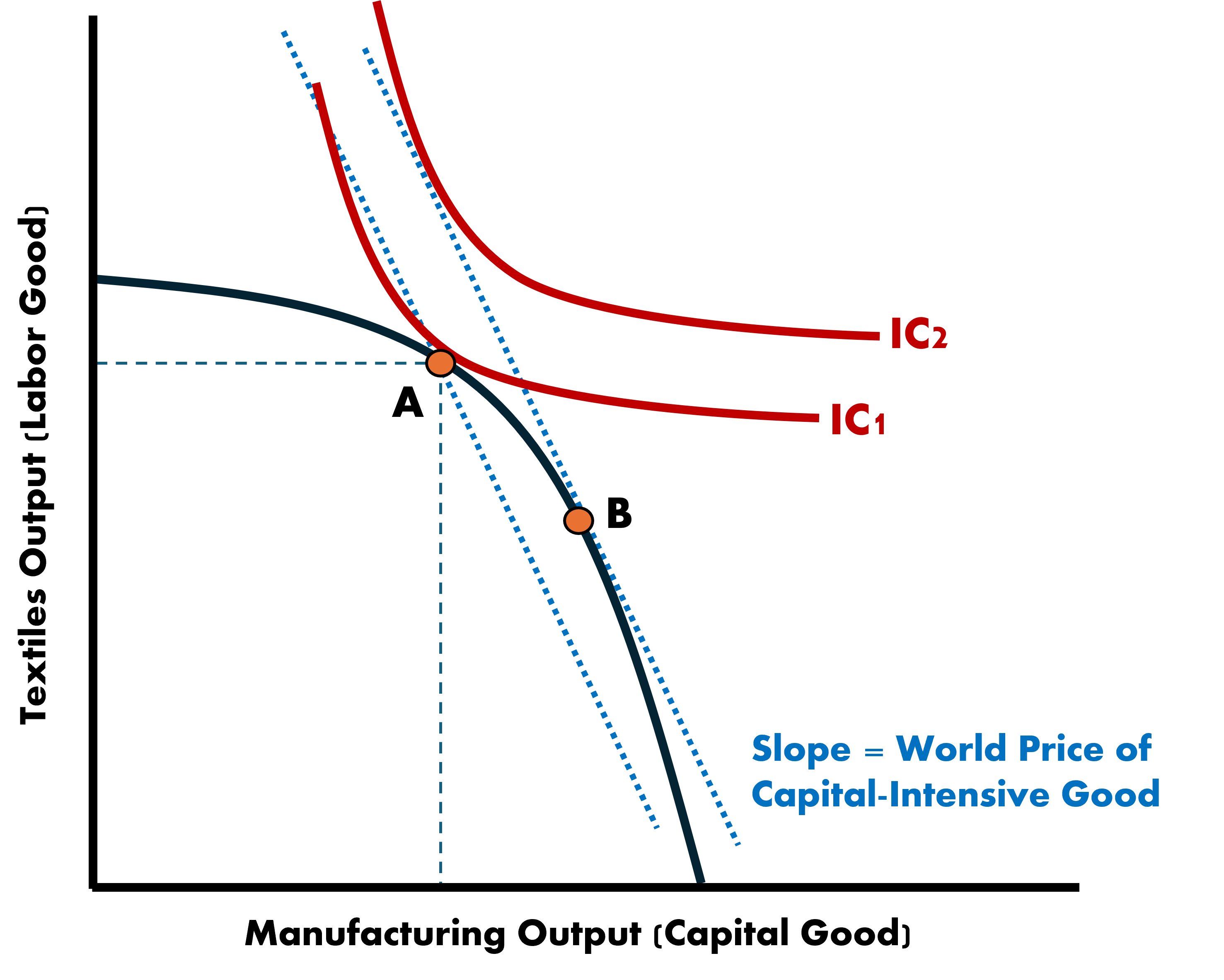
Free Trade - Gains from Trade

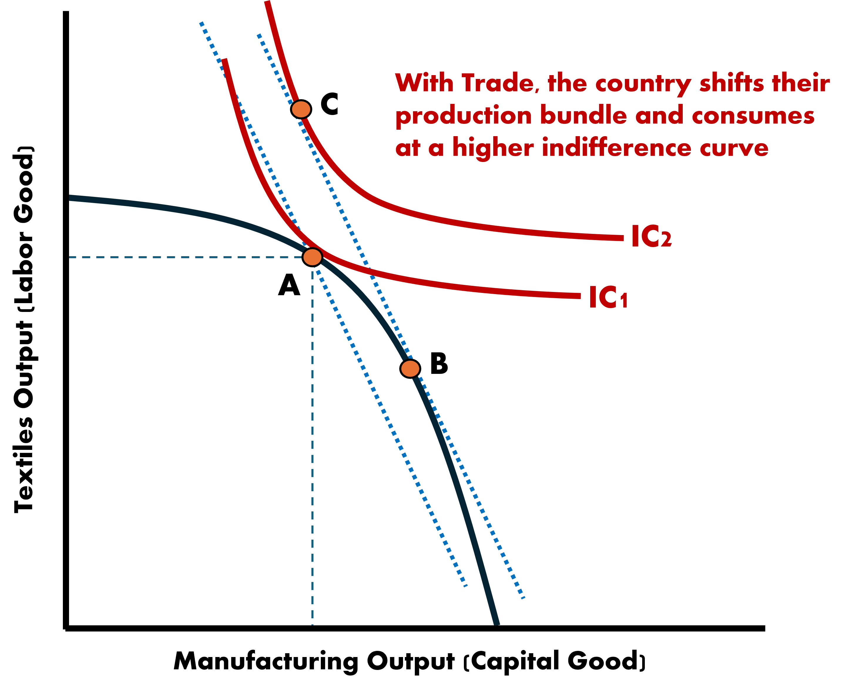
Gains from Free Trade

Since we are trading at the world price level, we can reach higher indifference curves

• The country produces at B and consumes at C

Therefore if the country produces more of the capital-intensive product than they consume, the must be exporting a subset of that good

• That is the difference between bundle B and bundle C

In constrast, the country produces less textiles than they consume, which suggests that they are importing the difference

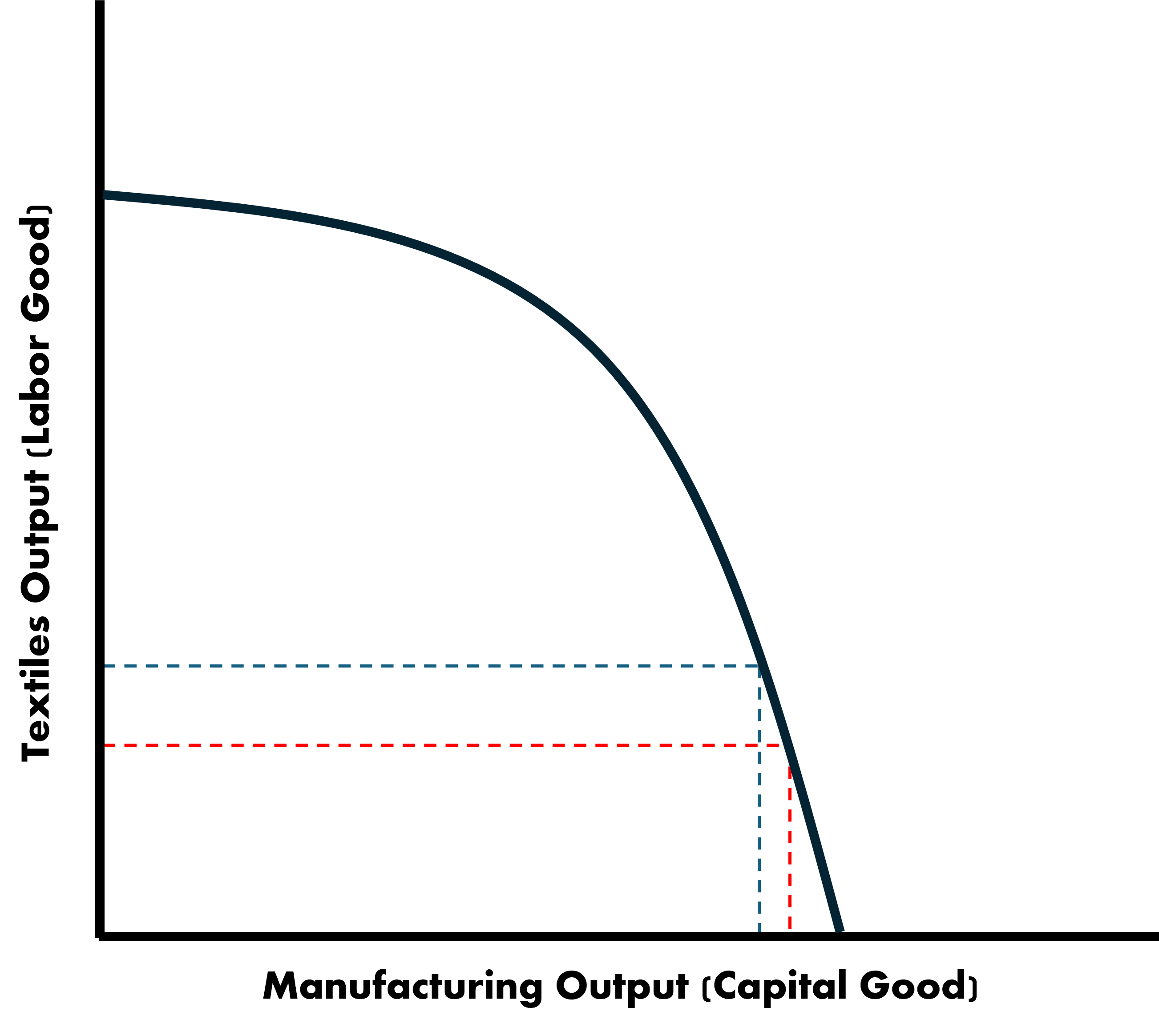
Comparing to the Ricardian Model

Try to remember why a country would shift their production when trading under a different world price

The country must produce where the opportunity cost is equal to the relative world price slope

The gains from trade are very similar between both models

Except that the specialization in production is not complete

• This is due to diminishing marginal productivity associated with each factor

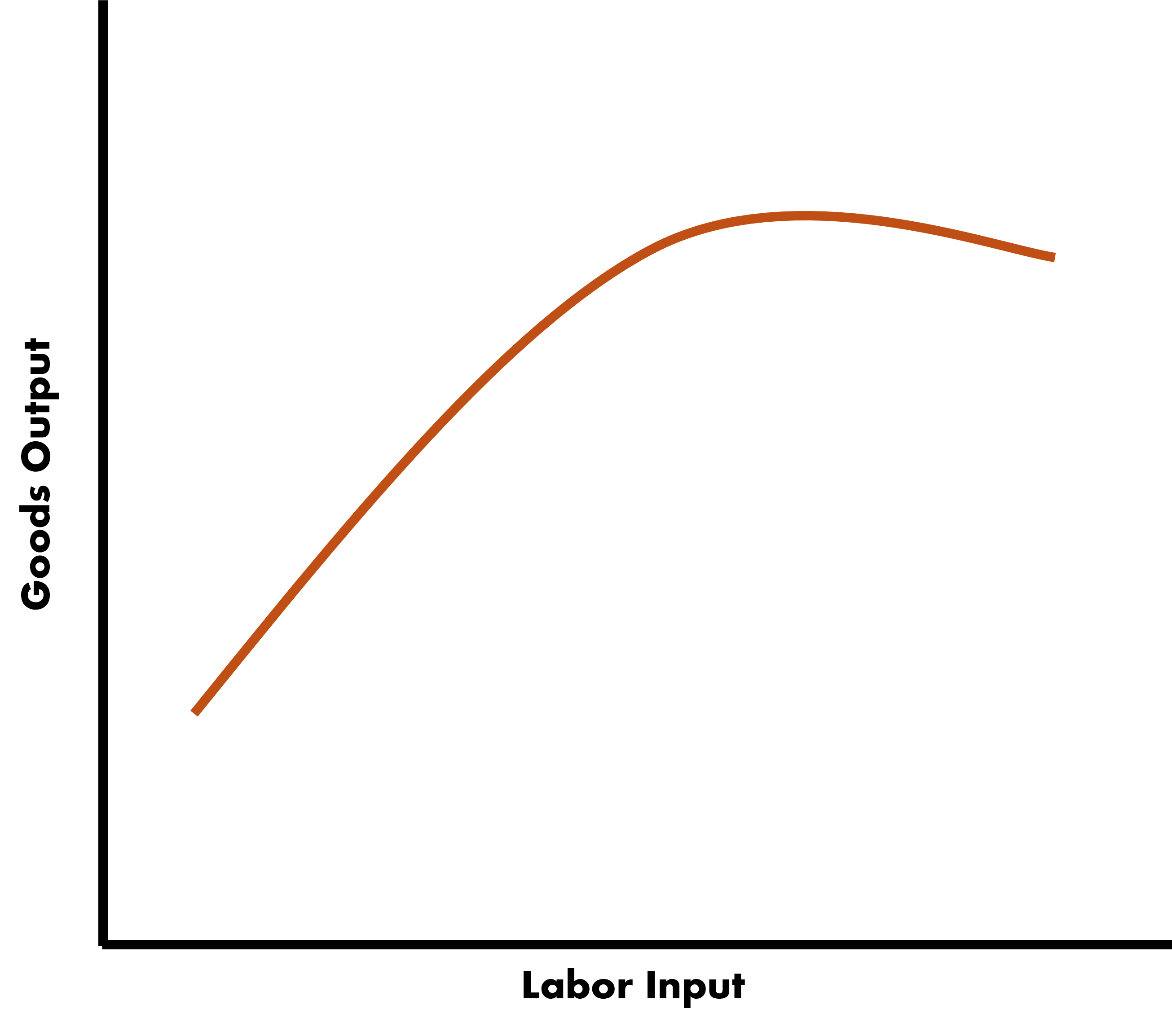
Diminishing Marginal Productivity

Definition: Holding the other factor(s) fixed, the marginal unit increase of a given factor yields an increasingly smaller contributions to overall output

Imagine having one shovel to share between 5 workers. The workers can take turns with the shovel whenever they get tired. But how much could total work output increase if we add 10 more workers?

Not much

Diminishing Marginal Productivity

Diminishing Marginal Product of Labor

Trade & Income Distribution

In the Ricardian Model we ruled out harmful effects and suggest everyone benefits in society. Reallocated workers simply leave the shrinking industry for an expanding one.

They are able to exchange their unchanged labor supply for a larger bundle of goods

• Specialization doesn’t incur any costs/penalties

The HO Model takes a more moderate view

Rather than capital and labor, let’s consider two labor sectors:

• Skilled

• Unskilled

Industries require different combinations of skilled and unskilled labor

Heterogenous Income Effects

We will go into this further later in the course but for now let’s keep in mind that trade openness can have heterogeneous effects depending on which part of the skill bracket the worker belongs to

It can be shown that a systematic relationship exists between endowments of factors for a country and who ends up being winners and losers

I’ll show you a theoretical argument for how this can happen. Later we will look at empirical evidence, which uses applied econometric analysis.

Stolper-Samuelson Theorem

Theoretical Outcomes of Assymetric Factors

The Stolper-Samuelson Theorem states that:

• Income depends on input supplied to the value of final product
• Wages will vary depending on their skill level
• Labor input earnings (wages) demand on their demand and supply

Derived Demand: Indirectly finding demand of an input used in produciton from the demand of the final good

If a good is in high demand, and therefore its price is high, then input factors receive high returns

Changes in Prices & Effects on Income

Any change that impact prices will have direct impacts on outcomes

• Open trade causes the export good price to rise and import good price to fall

• Demand for each input factor readjusts, which leads to changes in returns to each factor

• Resources shift away from the imported good sector and move toward the exported good sector, which cause changes in demand for each input

Stolper-Samuelson Example

Let’s consider an economy where the sports cars are the export good

These require a high amount of capital and low amount of labor inputs

Because it is the export good, demand for capital factors rise and demand for labor factors fall

This implies that income for factors in higher demand will rise

Income for factors in lower demand will fall

Stolper-Samuelson Theorem suggests that the increase in price of a good raises the income earned by factors intensively used in its production. A fall in price of a good lowers the income of factors used intensively

Stopler-Samuelson Theorem

According to this theory, a country with a capital-intensive presence (like the US) will shift away from labor demand

• Capital owners will benefit from trade
• Labor will lose out

There is an extension to this called the Magnification Effect which says that changes in prices lead to a larger change in factor incomes

Magnification Effect

Let’s look at how this works in theory

Recall the Stopler-Samuelson Theorem: When the Price of a good increases, the income earned by the factor intensively used in production will increase. The other factor will see decreased earnings.

We can write this up mathematically:

\[ P_{X} = \alpha_{L} * w + \alpha_{K} * r \]

Where

• \(\alpha_{L}\): Labor Share of Factor Inputs
• \(\alpha_{K}\): Capital Share of Factor Inputs

• \(w\): Wage Rate of Labor
• \(r\): Rental Rate of Capital

Magnification Effect

\[ P_{X} = \alpha_{L} * w + \alpha_{K} * r \]

Let \(\alpha_{L}\) be 0.25 and \(\alpha_{K}\) be 0.75

Then this product is made 25% by labor and 75% by capital inputs

It is capital-intensive

The Stolper-Samuelson Theorem predicts that if \(P_{X}\) increases, then \(r \uparrow\) and \(w \downarrow\)

The Magnification Effect says that if prices go up by, let’s say, 10%, then the capital rental rate will see earnings increase by more than 10%

Magnification Effect - Example

Let’s introduce some notation:

\[ \Delta P_{X} = \alpha_{L} * \Delta w + \alpha_{K} * \Delta r \]

Here the \(\Delta\) means “change in”

Let’s throw some numbers to see it in action

\[ 10 \% = 0.25 * -5\% + 0.75 * \Delta r \]

\[\begin{align} 10 \% &= - 1.25 \% + 0.75 * \Delta r \\ 10 \% + 1.25 \% &= 0.75 * \Delta r \\ 11.25 \% &= 0.75 * \Delta r \\ \dfrac{11.25}{0.75} \% &= \Delta r = 15 \end{align}\]

Bridging the Gap in Time

Movement across sectors and optimization of production occurs in what we generally call the Long-Run

The Long-Run is an arbitrary amount of time. It is used as a measure of how things work out after all possible adjustments/adaptations occur.

Let’s look at an example:

Suppose world prices adjust to trade openness and labor resources begin leaving the US steel industry toward some other industry

In the Long-Run, workers may retrain and find employment elsewhere but in the Short-Run they are stuck with pay cuts and unemployment

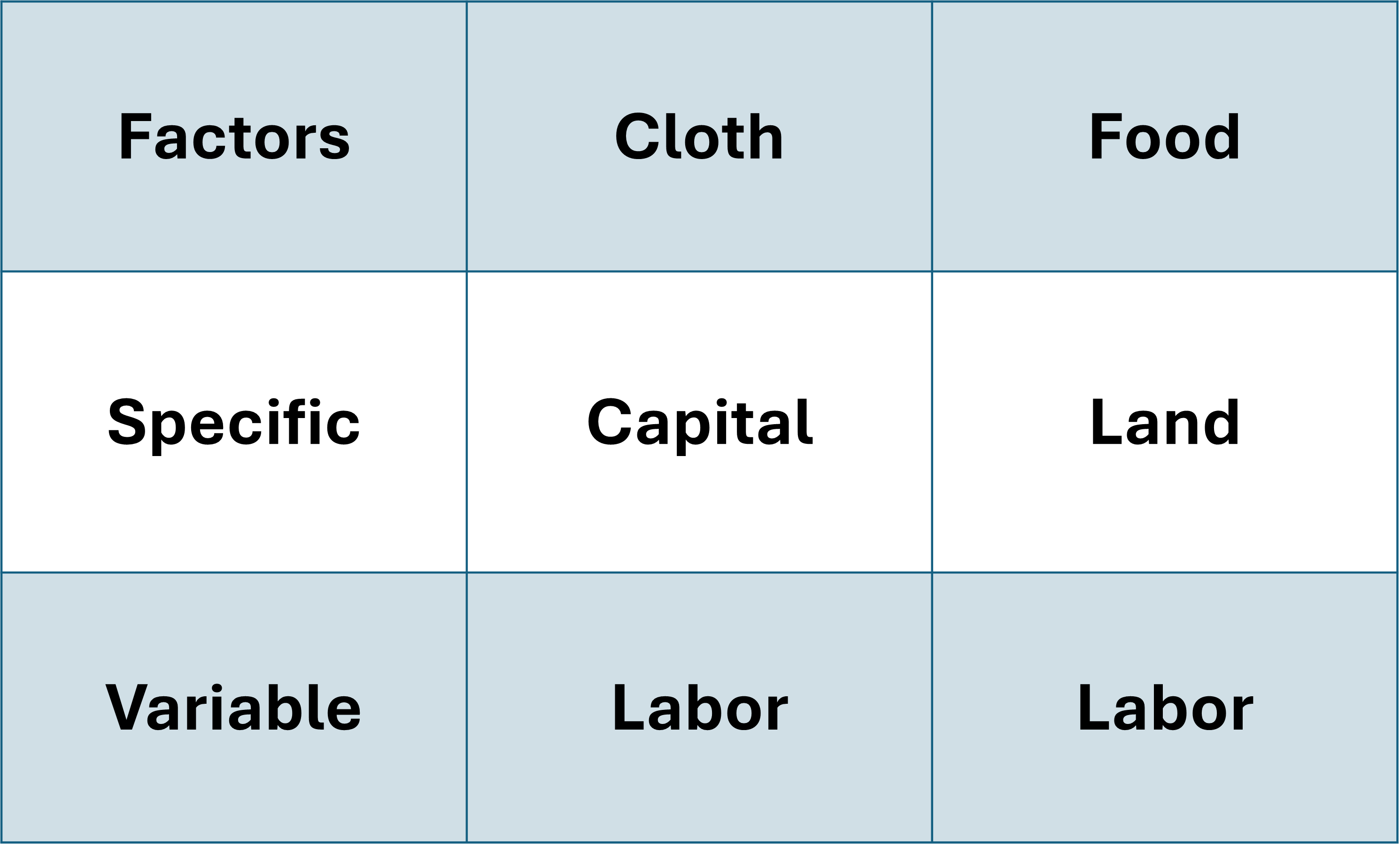
Specific Factors Model

Heterogeneity Across Time

We can consider the Short-Run stickiness in our HO Model by adding some conditions:

• Three Input Factors: Labor (L), Capital (K), Land (T)
• Two Goods: Cloth and Food
• Production Functions:
  • \(Q_{c} = f(K, L_{c}) \Rightarrow \;\) Cloth is made with Capital and Labor employed in Cloth
  • \(Q_{f} = f(T, L_{f}) \Rightarrow \;\) Food is made with Land and Labor employed in Food
  • Labor across industries must sum up to total labor: \(L = L_{c} + L_{f}\)

Specific and Variable Factors

We call Labor our variable factor because it is used in the production of both goods

And Land and Capital are specific factors because they are exclusively used for specific goods

With these modifications to the HO Model, we have now extended it into a Specific Factors Model

Specific Factors are immobile

• They cannot move between the two industries

Variable Factors are mobile

• Labor can freely move across industries

Trade Patterns

Trade flows will be determined similarly to our HO Model

The difference is that Specific Factors will play a key role in determining Comparative Advantages

Trade flows will be determined by the relative endowment of the Specific Factors

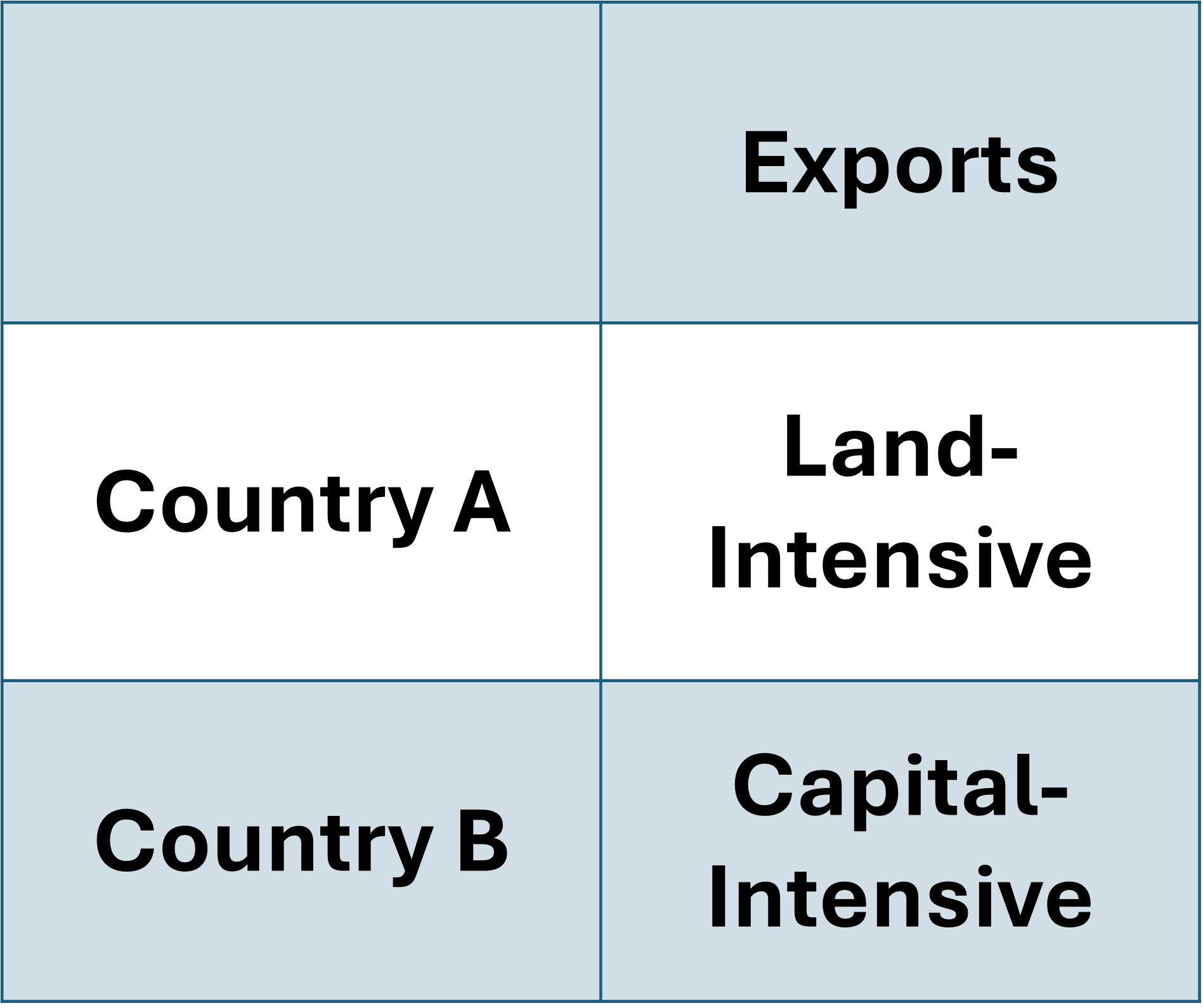
Trade Patterns

Let’s say that Country A is relatively well endowed with land and Country B is relatively well endowed with capital

Country A will Export

• Food

Country B will Export

• Cloth

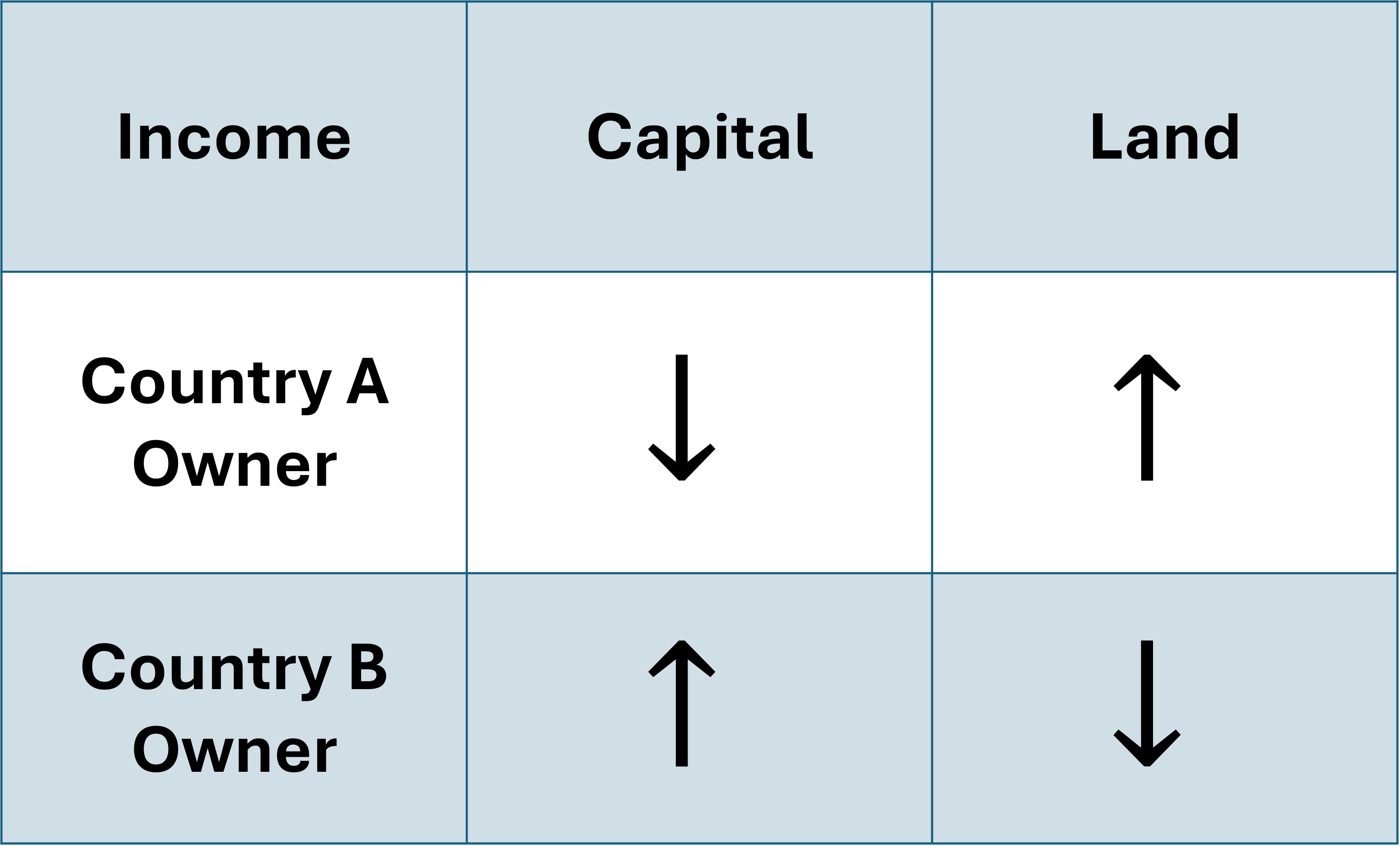
Specific Factors Dynamics

Let’s look at the steps of openning to trade:

• Each country opens up to trade
• They each follow their comparative advantage and move toward greater specialization
• The shift in production reduces demand for the specific factor used in the non-specialized industry
  • In our example, the demand for capital in Country A goes down
• Income for the less utilized specific factor also declines

Specific Factors Dynamics

This model helps us view income distribution effects of trade more clearly

So we have Country A capital owners be hurt, due to the economy moving away from production of capital-intensive cloth

On the other hand, we have Country A landowners experience the opposite effect

Specific Factors Dynamics

How about Labor?

Because labor is mobile between industries, workers that are laid off in the declining sector will find employment in the expanding sector

Additionally, prices of both goods shift from what they were under autarky

In Country A where Food is the export, we would see:

Price of Food

Increase!

Price of Cloth

Decrease!

Ask why \(\rightarrow\) because world price for export is higher than at home and import is lower than at home

Effects on Variable Factor Income

The income distribution effect on the variable good is ambiguous

• The net effect depends on which is strongest, rising Food prices or falling Cloth prices

• It also on their consumption patterns

In its most basic form, we have adapted the HO Model in such a way that we can observe income distribution effects:

• Across factor inputs that are specific to production (Specific Factors)

• Within factors used in both forms of production (Variable Factors)

Extensions to Trade Theory

Empirical Tests

So far we have argued in-favor and against gains from trade exclusively from theory

You should always be skeptical and ask yourself two questions:

• Do the predictions of generalized models hold in the real world?

• Are there other reasons that these predicted patterns may be observed in the data?

A great deal of work that economists do is translating theory into empirical analysis

For example, Blonigen & Wilson (2008) examine whether port efficiency allows for greater volume of trade

Emperical Tests - Comparative Advantage

All trade theories come down to differences between countries that establish comparative advantages which motivate trade

Each theory predicts which goods a country will import and export

Empirical tests are difficult due to our inability to observe an ‘autarky’ counterfactual and difficulty in measuring factor endowments

Rather than going between extremes of no-trade to completely free trade, we normally imagine changes in trade openness as a result of:

• Lower tariff rates and reduced trade quotas

Theory vs Empirics

Ricardian Model

• Challenging to test due to the assumption of relative differences in technology augmenting labor productivity

• Most countries do not produce goods for which they are at a comparative disadvantage so there is no way to measure their productivity in those sectors

Findings

• As labor producitity in a particular industry rises, the intensive margin by which goods are exported increases. The country becomes a net exporter of that godo

The Ricardian model has been more frequently and succesfully tested

Theory vs Empirics

HO Model

• Even harder to apply tests due to challenges involved in accurately measuring factor endowments. Our measures of land and capital values are imprecise estimates

Findings

• Cross-country measures of capital, land, and labor endowments are often measured using different means due to methodological differences across national accounting bodies

• Even with these flaws, the HO Model is a useful starting point through factor endowments which can then be supplmented with other ideas

• Useful way to categorize the income distribution effects of trade

Other important determinants of trade such as economies of scale, corporate structure, and economic policy are not considered in the model

Findings: Housing’s contributions to CPI is based on mortgage values in Europe while the US uses a rental-equivalence approach

Empirical Tests

So how do we address international economic theories when countries are all measuring our key statistics in different ways?

This normally requires an Non-Governmental Organization (NGO) or world body to apply data collection methods in a cross-country manner

For example, I used data from UN Comtrade which contained values of trade between countries at a detailed level

I complemented this with political manifesto data provided by the Comparative Manifesto Project in order to document how increased opennes to trade has shifted political leans in Costa Rica

Empirical Tests

Other differences between countries, beyond technology and factor endowments, that partly explain difference in trade flows across countries are:

• Economies of Scale

• Corporate structures

• Economic policy

• Public infrastructure

• Institutional quality

Extensions to Trade Theory

Because of these empirical concerns and other key country-level differences, further extensions to HO have been developed

• Gravity Model
• Product Cycle

• Trade vs FDI
• Offshoring & Outsorcing
  

These provide theoretical settings which explain a portion of existing trade

Extension - Gravity Model

This model says that to explain how a country trades with other countries, we must factor in distance and size

• The larger the other country is, the more demand it represents on the global market for a given good

• The closer the other country is, the cheaper it is to access that market

\[ T_{ij} = \dfrac{GDP_{i}^{\alpha} * GDP_{j}^{\beta}}{D_{ij}^{\theta}} \]

Many empirical analyses leverage model specifications on these key factors, which explain much of the variation obseved in country-level trade flows

Extension - Gravity Model

Some examples to fix ideas:

• Mexico’s most important trade partner is the US

  • Distance: Share a border which means transport costs are less than, let’s say, Europe
  • Market Size: US market is huge, and will absorb a lot of Mexican output

• US trade with Korea vs trade with Japan

  • Distance: Relatively same distance which means equal-ish transport costs
  • Market Size: Japanese economy is larger which means more US goods enter Japan relative to Korea

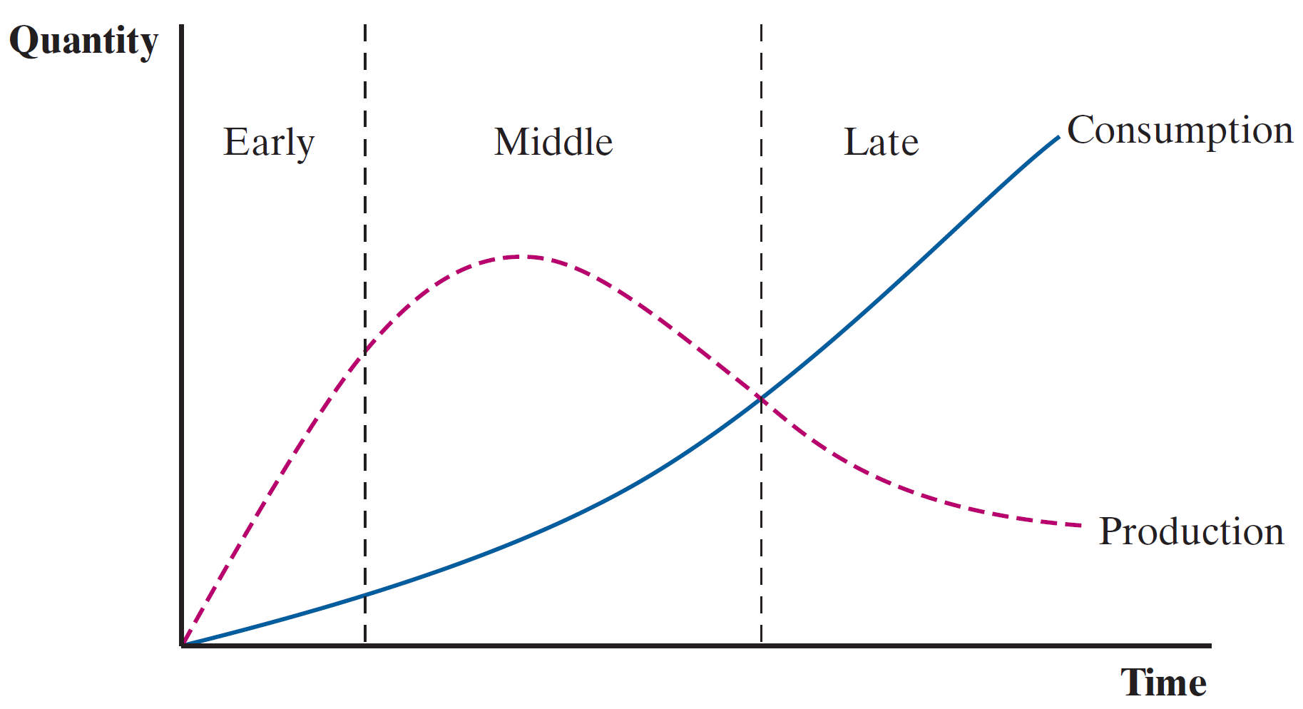
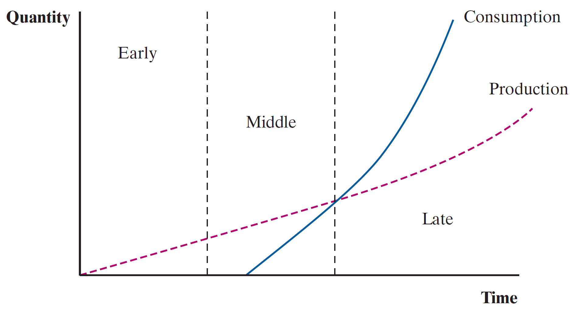
Extension - Product Cycle

Explains exports of sophisticated manufactured goods from countries who are scarce in skilled labor and capital

Many manufactured goods go through product cycles where factor inputs change over time

Early/Development

Middle/Standardized

Late

Extension - Product Cycle

Early/Development

• Goods are produced with a lot of testing (in inputs and final form)
  • Requires skilled labor to promote and develop product
• Consumers with higher incomes will be early-adopters and provide crucial feedback

Extension - Product Cycle

Middle/Standardized

• Product becomes standardized in characteristics and production process
• Shift production toward low labor cost nations

Extension - Product Cycle

Late

• Consumption in high-income countries exceeds production
• Production is concentrated in low-income countries as production process has taken form of assembly-type operations
• High-income countries need to innovate and restart the cycle in order to continue growth

Extension - Product Cycle

High-Income Countries

Low-Income Countries

The composition of factor inputs and cost minimization decisions by firms lead to relocation of production efforts, increasingly toward lower-cost labor nations

Trade/FDI

In the Product Cycle extension, firms invest abroad and some output generated is sent home for consumption

• This is a great difference from the HO Model where no investment abroad is taken into consideration and factor endowments cannot cross countries

• We can then introduce the concept of Foreign Direct Investment (FDI)

FDI suggests that cases may exist where firms elect to invest abroad rather than transport/ship goods abroad

Intrafirm trade is when these firms, with foreign affiliates, import outputs back home and it is handled by the parent firm

Extension - Offshore/Outsorce

Offshoring: Set up a plant abroad to produce goods

Outsorcing: Contract a different firm to produce goods for you. Can be international.

Modernization of the trade process has made these international features of production and distribution chains more feasible

• Largely driven in the 1990s by internet availability, satellite communication, containerization of cargo and improved computing power

• Easier to succesfully manage business operations abroad (marginal cost of multinational enterprise operations lower)

Extension - Offshore/Outsource

Effects include a trend toward international production, with comparative advantages across countries featuring in individual firms’ supply chains

Rather than specialize in goods, countries can specialize in key intermediate inputs

Trade economists refer to this as increased formations of global value chains

Many exports and local production processes now rely on the availability of imports

There is a huge vulnerability if ports become congested or delays occur

Next Topics

Issues in Trade and Empirical Evidence

Reading

• Second Part of Ch 4

Read Abstract, Introduction and Conclusion

• Autor et al (2013) - China Shock Syndrome

• Autor et al (2020) - Importing Political Polarization

Assignments

• Problem Set 02